Calibrated Model
These instructions describe how to run and analyze the archived calibrated model.
Startup an R session. Set the working directory to the local wrv-training repository, that is the “wrv-training” folder, by typing the following command in your R console and making sure to change the file path to the correct location:
setwd("C:/Users/jfisher/Repos/wrv-training")Load the wrv, inlmisc, raster, and leaflet packages into your current R environment, using
packages <- c("wrv", "inlmisc", "raster", "leaflet")
lapply(packages, library, character.only = TRUE)
Get Model Input Files
Download model input files for the calibrated model, these files were archived on the USGS Water Resources NSDI Node. Use the following commands to write model input files to the “archive” folder in your working directory.
url <- "https://water.usgs.gov/GIS/dsdl/gwmodels/SIR2016-5080/model.zip"
file <- file.path(tempdir(), basename(url))
download.file(url, file)
files <- unzip(file, exdir = tempdir())
files <- files[basename(files) != "usgs.model.reference"]
file.copy(files, "archive", overwrite = TRUE)
Four additional files are included in the “archive” folder but are not required for running the calibrated model. The “eff.csv”, “seep.csv”, and “trib.csv” text files contain the calibrated values of irrigation efficiency, canal seepage, and tributary underflow, respectively. And the “model.rda” binary file contains R objects d.in.mv.ave, misc, reduction, rs, ss.stress.periods, tr.stress.periods, and trib. A description of each of these R objects is given in the help documentation of the UpdateWaterBudget function in the wrv package, accessed using
help("UpdateWaterBudget", package = "wrv")Load R objects stored in the R-data file (“archive/model.rda”) into your current R environment using the following command:
load("archive/model.rda")Note that the rs object contains multiple raster images describing the geometry of the model grid, and is used throughout these instructions.
Calculate Transmissivity
Transmissivity is a measure of how much water can be transmitted horizontally, such as to a pumping well. To calculate transmissivity values in model layer 1, multiply the layer thickness by the calibrated hydraulic conductivity. Recall that a specified-thickness approximation was made in model construction, in other words, the saturated thickness is assumed to be independent from head changes in the aquifer system. Therefore, we can get away with using layer thickness rather than saturated thickness in layer 1.
Write a simple function to read model input reference files (“*.ref”).
ReadReferenceFile <- function(file, mask.value = 1e+09) {
  x <- scan(file, quiet = TRUE)
  x[x == mask.value] <- NA
  r <- raster(rs)
  r[] <- x
  return(r)
}
Put our new function to use by reading in the calibrated hydraulic conductivity values.
r <- ReadReferenceFile("archive/hk1.ref")
names(r) <- "lay1.hk"
rs <- stack(rs, r)
r <- ReadReferenceFile("archive/hk2.ref")
names(r) <- "lay2.hk"
rs <- stack(rs, r)
r <- ReadReferenceFile("archive/hk3.ref")
names(r) <- "lay3.hk"
rs <- stack(rs, r)
Calculate the transmissivity of model layer 1.
r <- (rs[["lay1.top"]] - rs[["lay1.bot"]]) * rs[["lay1.hk"]]Finally, draw a map of transmissivity in model layer 1.
r[] <- log10(r[])
Pal <- colorRampPalette(c("#F02311", "#FFFFEA", "#107FC9"))
usr <- c(2451504, 2497815, 1342484, 1402354)
breaks <- pretty(r[], n = 15, na.rm = TRUE)
at <- breaks[c(TRUE, FALSE)]
labels <- ToScientific(10^at, digits = 1, lab.type = "plotmath")
credit <- paste("Base derived from U.S. Geological Survey National",
                "Elevation Dataset 10-meter digital elevation model.\n",
                "Idaho Transverse Mercator projection;",
                "North American Datum of 1983.")
explanation <- paste("Transmissivity, in square meters per day,",
                     "plotted on a logarithmic scale.")
PlotMap(r, breaks = breaks, xlim = usr[1:2], ylim = usr[3:4],
        bg.image = hill.shading, bg.image.alpha = 0.6, dms.tick = TRUE,
        pal = Pal, explanation = explanation,
        rivers = list(x = streams.rivers), lakes = list(x = lakes),
        labels = list(at = at, labels = labels), credit = credit,
        contour.lines = list(col = "#1F1F1F"), scale.loc = "bottomleft")
plot(cities, pch = 15, cex = 0.8, col = "#333333", add = TRUE)
text(cities, labels = cities@data$FEATURE_NA, col = "#333333", cex = 0.5,
     pos = 1, offset = 0.4)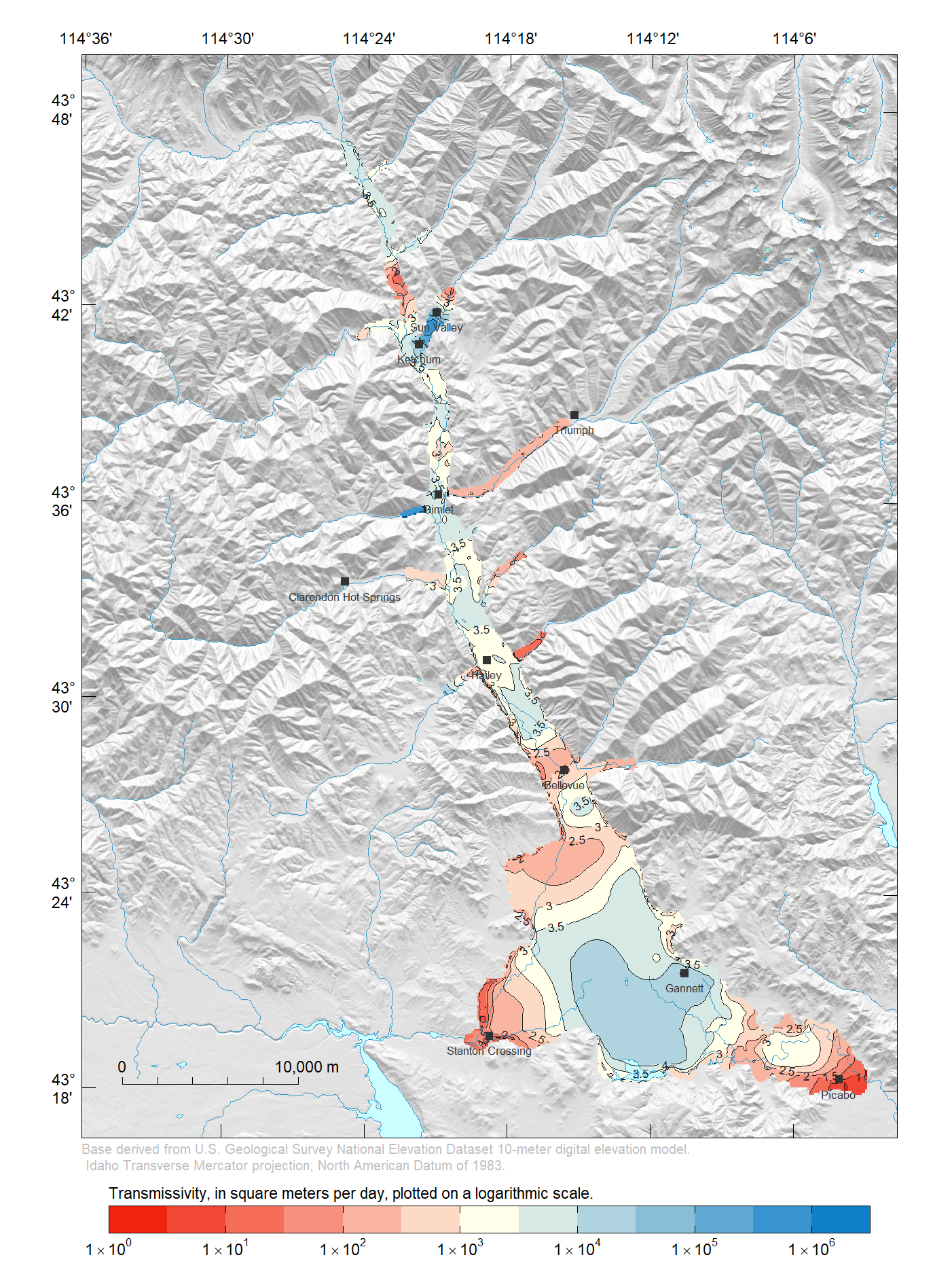
Recalculate Specified Flows
Recalculate the specified-flow boundary conditions for the groundwater-flow model. These boundary conditions include: (1) natural and incidental groundwater recharge at the water table, (2) groundwater pumping at production wells, and (3) groundwater underflow in the major tributary valleys. Specified-flow values are saved to disk by rewriting the MODFLOW Well Package file (“archive/wrv_mfusg.wel”).
UpdateWaterBudget("archive", "wrv_mfusg", qa.tables = "english")Because no changes were made to the model input files, the MODFLOW Well Package file remains the same, with one exception. An option is set that indicates to MODFLOW that cell-by-cell flow terms should be written to disk—a requirement for post-processing the simulated water budget. Recalculating the specified flows also results in quality assurance tables being written to disk ("archive/qa-*.csv").
Run MODFLOW
Copy the MODFLOW-USG executable file from the wrv package to the “archive” folder—the executable will be compatible with your operating system. Note that the executable version has been updated from 1.2, included in the model archive, to 1.3.
file.name <- ifelse(.Platform$OS.type == "windows", "mfusg.exe", "mfusg")
arch <- ifelse(Sys.getenv("R_ARCH") == "/x64", "x64", "i386")
file <- file.path(system.file("bin", arch, package = "wrv"), file.name)
file.copy(file, "archive", overwrite = TRUE)
Create a batch file (“archive/RunModflow.bat”) containing an OS command that will run MODFLOW-USG.
cat("mfusg \"wrv_mfusg.nam\"", file = "archive/RunModflow.bat")Run MODFLOW-USG by either double-clicking the batch file (“archive/RunModflow.bat”) in File Explorer, or pasting the following commands into your R console:
wd <- setwd("archive")
system2(file.path(getwd(), "RunModflow.bat"), stdout = FALSE, stderr = FALSE)
setwd(wd)
Post-Process Model
These instructions describe an example analysis of model output.
View head distribution
Read simulated hydraulic head (head) values for the calibrated model, located in “archive” folder.
heads <- ReadModflowBinary("archive/wrv_mfusg.hds")
dates <- as.Date(vapply(heads, function(i) i$totim, 0),
                 origin = tr.stress.periods[1])
layer <- vapply(heads, function(i) i$layer, 0L)
FUN <- function(i) {return(setValues(raster(rs), i$d))}
rs.heads.lay1 <- mask(stack(lapply(heads[layer == 1L], FUN)), rs[["lay1.bot"]])
rs.heads.lay2 <- mask(stack(lapply(heads[layer == 2L], FUN)), rs[["lay2.bot"]])
rs.heads.lay3 <- mask(stack(lapply(heads[layer == 3L], FUN)), rs[["lay3.bot"]])
raster.names <- format(dates[layer == 1L])
names(rs.heads.lay1) <- raster.names
names(rs.heads.lay2) <- raster.names
names(rs.heads.lay3) <- raster.names
Choose a model time step to view the simulated head distribution. The following command prints the date corresponding to each time step:
print(names(rs.heads.lay1))We arbitrarily decided to view the spatial distribution of head on August 8, 2007.
sim.date <- "2007-08-01"  # date format is YYYY-MM-DD
rs.head <- stack(rs.heads.lay1[[sim.date]],
                 rs.heads.lay2[[sim.date]],
                 rs.heads.lay3[[sim.date]])
names(rs.head) <- c("lay1.head", "lay2.head", "lay3.head")
Define a transect line that will be used to view a vertical cross-section of simulated head values. The verticies of the transect line, expressed as latitude and longitude geographic coordinates, are specified using decimal degrees.
tran.ll <- rbind(c(-114.289069, 43.337289),
                 c(-114.228996, 43.350930),
                 c(-114.188843, 43.383649))
tran <- SpatialLines(list(Lines(list(Line(tran.ll)), ID = "Transect")),
                     proj4string = CRS("+proj=longlat +datum=WGS84"))
tran <- spTransform(tran, crs(hill.shading))
Draw a map of head in model layer 1 south of Bellevue, and include the line of cross section (B–B’).
r <- rs.head[["lay1.head"]]
usr <- c(2472304, 2497015, 1343284, 1358838)
r <- crop(r, extent(usr))
zlim <- range(pretty(range(r[], na.rm = TRUE)))
PlotMap(r, xlim = usr[1:2], ylim = usr[3:4], zlim = zlim,
        bg.image = hill.shading, bg.image.alpha = 0.6, dms.tick = TRUE,
        max.dev.dim = c(43, 56), credit = credit,
        rivers = list(x = streams.rivers), lakes = list(x = lakes),
        contour.lines = list(col = "#1F1F1F"), scale.loc = "bottomleft",
        explanation = "Hydraulic head, in meters above the NAVD 88")
lines(tran, col = "#F02311")
xy <- as(tran, "SpatialPoints")
text(xy[c(1, length(xy)), ], labels = c("B", "B'"), col = "#F02311",
     cex = 0.7, pos = c(2, 4), offset = 0.1, font = 4)
plot(cities, pch = 15, cex = 0.8, col = "#333333", add = TRUE)
text(cities, labels = cities@data$FEATURE_NA, col = "#333333",
     cex = 0.5, pos = 1, offset = 0.4)
legend("topright", c("Water-table contour", "Line of cross section"),
       col = c("#1F1F1F", "#F02311"), lty = 1, lwd = c(0.5, 1),
       inset = 0.02, cex = 0.7, box.lty = 1, box.lwd = 0.5, bg = "#FFFFFFCD")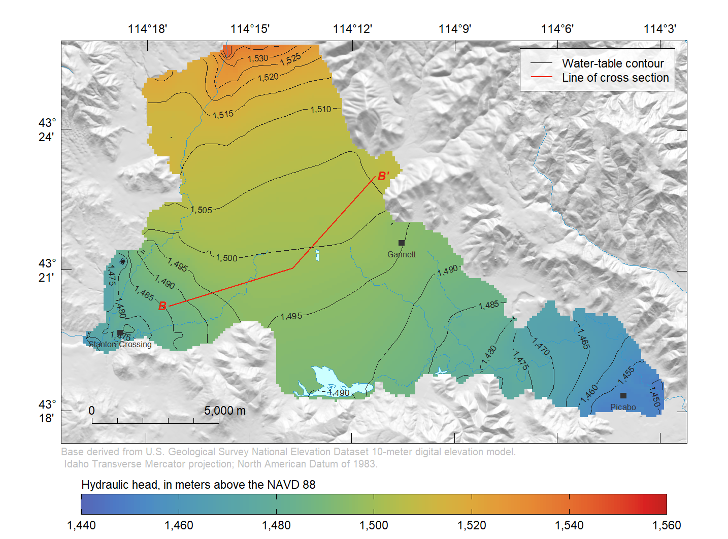
Finally, draw a vertical cross-section of simulated heads along the transect line B–B’.
PlotCrossSection(tran, stack(rs, rs.head),
                 geo.lays = c("lay1.top", "lay1.bot", "lay2.bot", "lay3.bot"),
                 val.lays = names(rs.head), wt.lay = "lay1.head", asp = 40,
                 ylab="Elevation, in meters above the NAVD 88",
                 explanation="Hydraulic head, in meters above the NAVD 88.",
                 contour.lines = list(col = "#1F1F1F"), draw.sep = FALSE,
                 unit = "METERS", id = c("B", "B'"), wt.col = "#3B80F4")
legend("bottomleft", c("Head contour", "Water table"),
       col = c("#1F1F1F", "#3B80F4"), lty = c(1, 1), lwd = c(0.5, 1),
inset = 0.02, cex = 0.7, box.lty = 1, box.lwd = 0.5, bg = "#FFFFFFCD")![]()
Compare head hydrographs
Aggregate each well’s spatial location, measured head, simulated head, and residual head data. This code chunk is a little complicated so don’t feel bad if you can’t follow along.
well <- obs.wells
head <- obs.wells.head
well.config <- GetWellConfig(rs, well, "PESTNAME")
FUN <- function(i) {
  idxs <- which(well.config$PESTNAME == i)
  return(max(well.config[idxs, "lay"]))
}
well@data$lay <- vapply(unique(well.config$PESTNAME), FUN, 0L)
head <- dplyr::left_join(head, well@data[, c("PESTNAME", "desc", "lay")],
                         by = "PESTNAME")
head$Date <- as.Date(head$DateTime)
head$head.obs <- head$Head
FUN <- function(i) {
  loc <- well[match(head$PESTNAME[i], well@data$PESTNAME), ]
  idx <- findInterval(head$Date[i], as.Date(raster.names), all.inside = TRUE)
  rs <- subset(get(paste0("rs.heads.lay", head$lay[i])), c(idx, idx + 1L))
  y <- extract(rs, loc)
  x <- as.numeric(as.Date(raster.names)[c(idx, idx + 1L)])
  return((y[2] - y[1]) / (x[2] - x[1]) * (as.numeric(head$Date[i]) - x[1]) + y[1])
}
head$head.sim <- vapply(seq_len(nrow(head)), FUN, 0)
head$head.res <- head$head.obs - head$head.sim
d <- aggregate(head[, c("head.obs", "head.sim", "head.res")],
               by = list(PESTNAME = head$PESTNAME), mean)
well@data <- dplyr::left_join(well@data, d, by = "PESTNAME")
Choose a single well from the groundwater observation network. We selected a well based on its USGS NWIS site number (SiteNo); although one could easily select it based on other well attributes, such as the IDWR site number (SITEIDIDWR), PEST identifier (PEST), common well name (WELLNUMBER), or its geographical coordinates. Draw the point locations of all observation wells within the aquifer system.
site.no <- "434104114241301"
w <- well[!grepl("driller well$", well$desc), ]
is.well <- w$SiteNo %in% site.no
crs <- CRS("+init=epsg:4326")
ll <- coordinates(spTransform(w, crs)); colnames(ll) <- NULL
file <- sprintf("markers/marker-%s.png", c("red", "blue"))
icon <- icons(iconUrl = ifelse(is.well, file[1], file[2]),
              iconWidth = 34, iconHeight = 34, iconAnchorX = 17, iconAnchorY = 34)
map <- CreateWebMap("Topo")
map <- setView(map, lng = ll[is.well, 1], lat = ll[is.well, 2], zoom = 13)
map <- addPolylines(map, data = spTransform(alluvium.extent, crs),
                    weight = 3, color = "#000000")
txt <- sprintf("<b>Site Number:</b> %s<br/><b>Site Name:</b> %s",
               w$SiteNo, w$WELLNUMBER)
map <- addMarkers(map, lng = ll[, 1], lat = ll[, 2], popup = txt, icon = icon)
map
Extract simulated and measured head data for selected well.
w <- well[well$SiteNo %in% site.no, ]
rb <- get(paste0("rs.heads.lay", w@data$lay))
ext <- t(extract(rb, coordinates(w)))
head.sim <- data.frame(Date = as.Date(rownames(ext)), head.sim = ext[, 1])
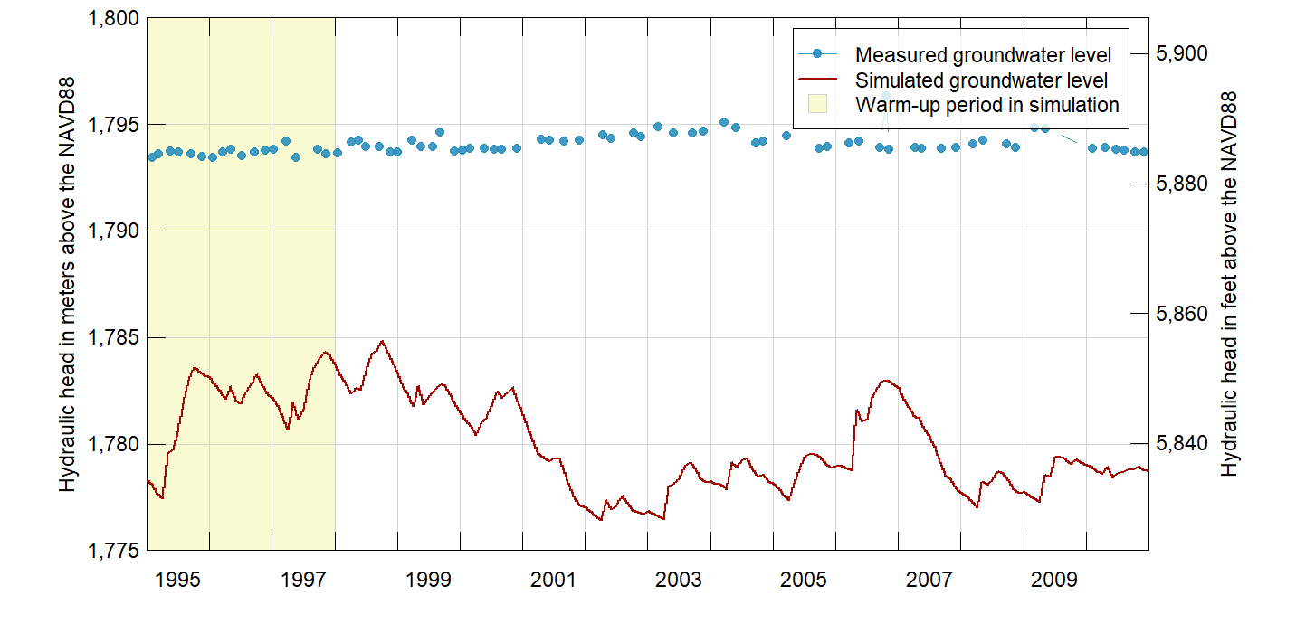
head.obs <- head[head$PESTNAME == w@data$PESTNAME, , drop = FALSE]Finally, plot the measured and simulated groundwater-level hydrographs. As the model report explains (p. 31), simulated hydraulic heads in the tributary canyons should be considered less reliable than in the main valley floor.
xlim <- range(head.sim$Date)
ylim <- range(pretty(range(c(head.sim$head.sim, head.obs$head.obs))))
cols <- c("#2A8FBDE5", "#A40802", "#FAFAD2")
xbuf <- as.Date(c("1995-01-01", "1998-01-01"))
bg.polygon <- list(x = xy.coords(c(xbuf, rev(xbuf)), c(rep(ylim[1], 2), rep(ylim[2], 2))),
                   col = cols[3])
ylab <- paste("Hydraulic head in", c("meters", "feet"), "above the NAVD88")
m.to.ft <- 3.280839895
PlotGraph(head.sim, xlim = xlim, ylim = ylim, ylab = ylab, col = cols[2],
          conversion.factor = m.to.ft, bg.polygon = bg.polygon,
          center.date.labels = TRUE, seq.date.by = "year")
lines(x = as.Date(head.obs$DateTime), y = head.obs$head.obs,
      type = "b", pch = 20, lwd = 0.5, col = cols[1])
labs <- c("Measured groundwater level", "Simulated groundwater level",
          "Warm-up period in simulation")
legend("topright", labs, pch = c(20, NA, 22), lwd = c(0.5, 1, NA),
       col = c(cols[1:2], "lightgray"), pt.bg = c(NA, NA, cols[3]),
       pt.lwd = c(NA, NA, 0.5), pt.cex = c(1, NA, 1.5), inset = 0.02,
       cex = 0.7, box.lty = 1, box.lwd = 0.5, xpd = NA, bg = "#FFFFFFCD")